Validation of TLMBHT to solve the Diffusion equation in time-domain for two-dimensions using Quadrangle elements
Feb 21, 2017 by Hugo Milan
Here, I will walk you through in how to use the TLM method to solve the Diffusion equation in 2D with the element Quadrangle by comparing the tlmbht predictions with analytical solution predictions.
Everything you need is available in the folder /vte/generalDiffusion/2D/QuadrangleNode. This folder was downloaded when you downloaded the source files. If you did not download the source files, you can download it from here. If you do not want to, you do not need to download or install anything–all the relevant outputs will be shown here. If you want to download tlmbht, go to releases and get the most updated version of tlmbht.
In this validation, we will follow the 5 steps showed here.
1) Create the geometry of the problem.
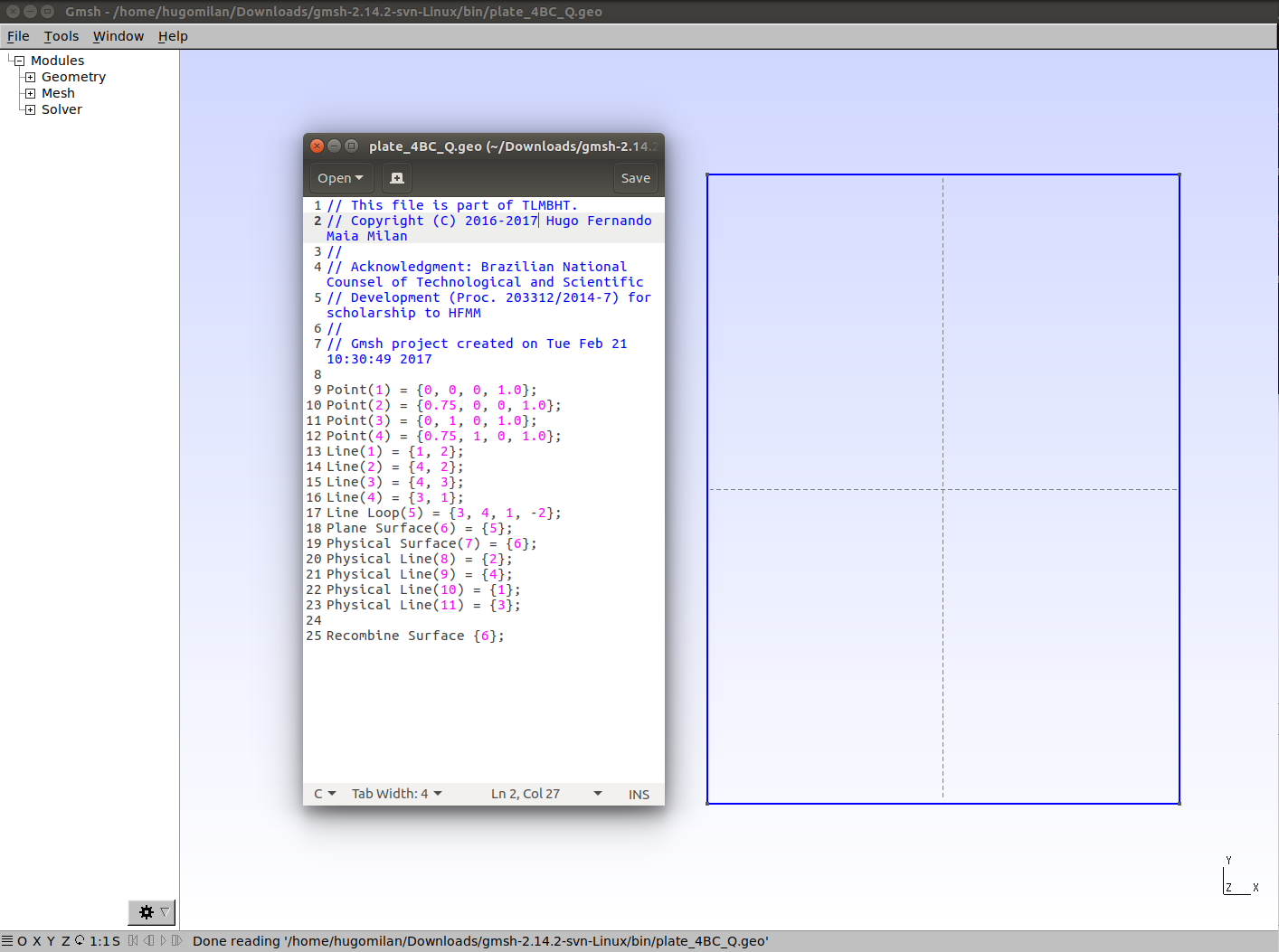
We are building up from the problem description of the validation for Diffusion 1D equation with line elements. Here, we will consider a simple two-dimensional problem that has analytical solution. In this problem, we will include source, two constant concentration boundary conditions (constant core concentration CC, and constant surface concentration CS), one constant flux boundary condition (qx), and one impermeable boundary condition. The problem geometry is shown below.

This geometry is a plate in a three-dimensional space, as you can see in the three-dimensional model below.
Now that we defined the problem, we need to draw the problem geometry using a format that tlmbht knows how to read. This was already done for you. The geometry of the problem was created using gmsh. The script file is plate_4BC_Q.geo. Note in the script file that we put ‘Physical tags’ in the Surface geometry and in the Lines. We did this so that we can tell tlmbht which tag is for material (number 7) and which tag is for boundary (number 8, 9, 10, and 11).

Now we are ready to create the mesh.
2) Create the mesh of the problem.
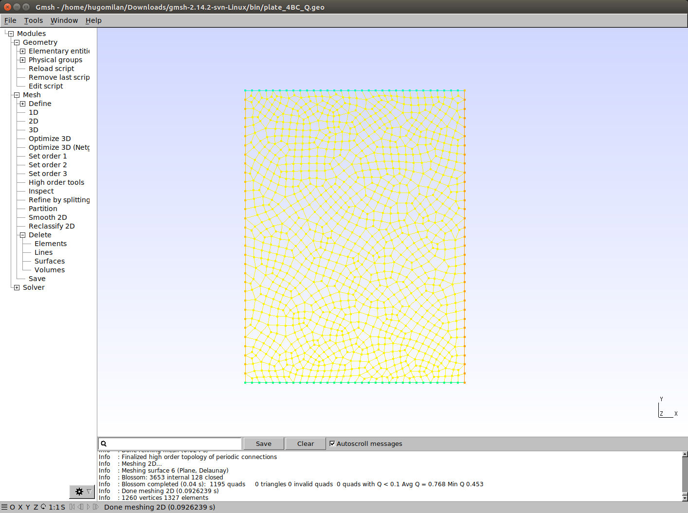
The mesh was easily created using gmsh/Mesh/2D and Refined by Splitting. The mesh file (already converted to tlmbht native mesh format) is plate_4BC_Q_1195e.tbn. It contains 1260 points (vertices), 128 line segments, and 1195 quadrangles (elements).

Now we are ready to create the description of the problem
3) Create the description of the problem.
The description of the problem is in the file cdiff2Qu.tlm. Here, I will explain how this case file was configured. However, if you are in a hurry, you can go skip this part and move on to the next section.
Explanation of this case file
The case file is structured in headers and I will go over every header in the file cdiff2Qu.tlm. This script file is similar to the script file for validation for Diffusion 1D equation with line elements. The differences are the inclusion of one additional boundary condition and changing to two-dimensions.
The first header you see (Simulation), is used to configure parameters common to the equations of the problem. In this case, we are only configuring the output extension to the ‘m’ (Octave/Matlab m format) so that it is easier to run the validation algorithm.
Simulation
{
    output extension = m;
}
The Mesh header contains information about the mesh. Here we tell the software which mesh to use (“file name”) and in what format it is (“input format”).
Mesh
{
    file name = plate_4BC_Q_1195e;
    input format = tlmtbn;
}
The Equation header tells the software what equation it should solve and how. You can have different Equations headers to defined different equations being solved simultaneously in a multi-physical problem. In the Equation header, we define the type of equation and give it a name. The name is essential to link what is in the Equation header with what is in the Material and Boundary headers. Then, we define the dimension of the problem and tell tlmbht to solve this problem in the time-domain (“Solve = dynamic”). Since we are solving a time-domain problem, we need to define the time-step and the final simulation time. The “time-jump” is a configuration that tells tlmbht after how many time-steps it should save the output data (which is defined in the “save” options). Here, we are saving at every 500 time-steps, which is equivalent to saving at every 5 s. Note that these 500 time-steps are all solved.
Equation
{
    type = diffusion;
    equation name = diffusion_name;
    dimensions = 2;
    Solve = dynamic;
    time-step = 1e-2;
    time-jump = 500;
    final time = 50;
    save = scalar;
    save = scalar between;
    save = vector;
}
The Material header defines the properties of the equation. You can have different Material headers for different properties in the same problem. We tell tlmbht to what equation this Material header is referred to by giving it the equation name (“diffusion_name”). In number, we give the Material header the Physical tag number that we gave to the elements during the mesh generation. Therefore, the options we input here are going to be applied to the elements that belong to the surface with tag number 7. Finally, we defined diffusion coefficient, volumetric source, and initial value (required for time-domain simulations).
Material
{
    equation = diffusion_name;
    number =  7;
    diffusion coefficient = 1e-9;
    source = 0.1;
    initial scalar = 20;
}
The Boundary header defines the boundary conditions. You can have different Boundary headers for different boundary conditions and for each equation being solved. We proceed similar to what we did in the Material header. That is, we define the equation name and the Physical tag number that this boundary will be applied to. For the boundary conditions to defined concentrations, we define the “scalar” options that tells tlmbht that these boundaries are for defined scalar (concentration, in this problem) values. For the boundary condition with defined flux, we define the “flux” option. We do not need to include the impermeable boundary condition because it is automatically applied to boundaries not defined by Boundary headers.
Boundary
{
    equation = diffusion_name;
    number = 10;
    scalar = 20;
}

Boundary
{
    equation = diffusion_name;
    number = 11;
    scalar = 50;
}

Boundary
{
    equation = diffusion_name;
    number = 8;
    flux = 1e-5;
}
The file cdiff2Qu_full.tlm contains additional explanation about the input. If you want more information in how to configure the case file, go to How to configure a case file.
4) Solve the problem.
Click here if you have Windows and need help to run tlmbht in your machine.
If you have the tlmbht binary in your path environment, simply type tlmbht cdiff2Qu.tlm. If you don’t have it in your path environment, you may copy the binary to the folder /vte/generalDiffusion/2D/QuadrangleNode/ and then type ./tlmbht cdiff2Qu.tlm. In some seconds, the calculation will be done.
If you want to see what is going on internally, you may run tlmbht with –verbose. If you want to see how long does it take to run tlmbht, you may run it with –timing. The command to run with both is simply tlmbht cdiff2Qu.tlm --verbose --timing.
Now we are ready to visualize the output and compare the TLM predictions with an analytical prediction.
5) Visualize the output.
After you have run tlmbht, it created the output file cdiff2Qu.m. In this tutorial, you do not need to worry about this file. We will run a script that automatically loads the data into Octave/Matlab. The script is in the file vdiff2Qu.m, which calls the analytical solver function D2_HEAT_f.m (click here to read more about the analytical solution and how to use this function).
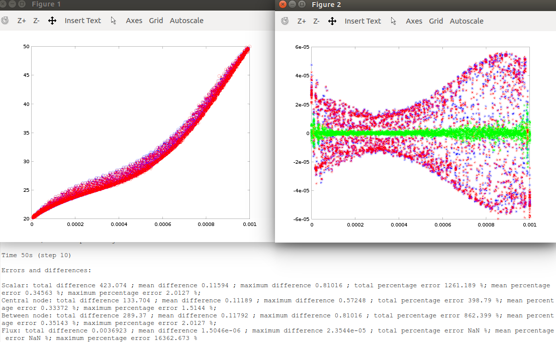
This part should be as simple as opening vdiff2Qu.m in Octave/Matlab and running it (press key F5). It will show you two plots and textual information. The figure below shows the two plots and part of the textual information. Concentration is shown in the left figure and flux is shown on the right figure. The analytical predictions are shown in blue, the tlmbht predictions are shown in red, and the green shows the difference of the calculated fluxes. In the concentration plots, asterisks represent concentration calculated at the center of the TLM nodes and the circles represent the concentration calculated between nodes. You can see that the predictions are almost identical, which you can confirm by looking at the textual information that tells you that the mean concentration error was 0.35 % and the mean flux difference was 1.5e-6 m-2 (which correspond to a fraction of 0.15 of the input flux). In this problem, we the mean flux error is not a viable validation variable because the flux is close to zero in some parts of the mesh and, hence, very small differences yields very large percentage errors. Moreover, concentration values close to zero inflated the percentage errors. However, we graphically observe that the tlmbht predictions match the analytical predictions very well.

You are not satisfied with this accuracy? Well… this is a numerical method; we will never get the same exact numbers as the analytical solution gives. Besides, this analytical solution is based on a infinity sum and, by default, the script vdiff2Qu.m only considers up to the first 100 terms. If you insist, you can try to increase the number of terms in the analytical solution. Then, as it is true for numerical methods, you can try to increase the number of elements and/or decrease the time-step. These changes will increase the computational time but also increase the accuracy.
What if the mesh was structured? The TLM theory works better with structured meshes. The file cdiff2Qu_S.tlm uses the structured mesh plate_4BC_Q_S_1024e.tbn and the predictions using this mesh had mean concentration error of 0.02 % and mean flux difference of 2.6e-8 m-2 (which corresponds to a fraction of 0.003 of the input flux).
Done!
I hope you have enjoyed this validation section! You may now try to change the case file (cdiff2Qu.tlm) and see what happens. Remember that if you change any parameter in the cdiff2Qu.tlm file you will need to do the same in the vdiff2Qu.m file. Except for time and space positions, they are not linked.
Remember: you are using a powerful numerical solver. You do not need to be constrained by solutions that can be solved analytically. Explore! Try different boundary conditions, include more materials, etc. Make this problem more realistic!
You might be wondering how does the tlmbht models for Triangle and Quadrangle elements change? They don’t change. These two validations solve the same problem. The only difference between them is that the mesh for the validation using Triangle elements has only triangles and the mesh for the validation using Quadrangle elements has only quadrangles. TLMBHT is capable of solving meshes that have any of these two elements.
Now, you can go to: