Analytical solution of the Diffusion/Heat equation in time-domain for three-dimensions

Jan 30, 2017 by Hugo Milan

You can download the algorithm D3_HEAT_f.m for Octave/Matlab that can solve this problem here and you can see instructions in how to use it here. If you want to see the final solution, go to Solution.

In this page, we will solve the dynamic diffusion/heat equation in three-dimensions using the principles of superposition and separation of variables. We build on the previous solution of the diffusion/heat equation in two-dimensions described here to solve this three-dimensional problem. The problem we will solve is restricted to the following initial and boundary conditions:

$\begin{matrix} C(x,y, z,t = 0) = C_{c} & \text{ or } & T(x,y,z, t = 0) = T_{c}\\ C(x,y = 0,z, t) = C_{c} & \text{ or } & T(x,y = 0,z, t) = T_{c}\\ C(x,y = H,z, t) = C_{s} & \text{ or } & T(x,y = H, z,t) = T_{s}\\ \dfrac{\partial C}{\partial x} (x = 0, y, z,t) = 0 & \text{ or } & \dfrac{\partial T}{\partial x}(x = 0, y, z,t) = 0\\ \dfrac{\partial C}{\partial x}(x = L, y, z,t) = \dfrac{q_x}{D} & \text{ or } & \dfrac{\partial T}{\partial x}(x = L, y, z,t) = \dfrac{q_x}{k}\\ \dfrac{\partial C}{\partial z} (x, y, z = 0,t) = 0 & \text{ or } & \dfrac{\partial T}{\partial z}(x, y, z=0,t) = 0\\ \dfrac{\partial C}{\partial z}(x, y, z = T_z,t) = \dfrac{q_z}{D} & \text{ or } & \dfrac{\partial T}{\partial z}(x, y, z = T_z,t) = \dfrac{q_z}{k} \end{matrix}$

The problem geometry for the heat equation can be represented as shown below. Geometry of the three-dimensional problem for diffusion equation

The problem geometry for the heat equation can be represented as shown below. Geometry of the three-dimensional problem for heat equation

This geometry is a parallelepiped in a three-dimensional space, as you can see in the three-dimensional model below.

Parallelepiped 0.75 x 1 x 0.375 by hugomilan on Sketchfab

Governing equations

Diffusion equation:

\begin{equation} \frac{\partial C}{\partial t} = D\left(\frac{\partial^2 C}{\partial x^2} + \frac{\partial^2 C}{\partial y^2} + \frac{\partial^2 C}{\partial z^2} \right) + S \end{equation}

where $C$ is concentration, $t$ is time, $D$ is diffusivity, and $S$ is source.

And we define the heat equation as:

\begin{equation} \rho c_{p}\frac{\partial T}{\partial t} = k\left( \frac{\partial^2 T}{\partial x^2} + \frac{\partial^2 T}{\partial y^2} + \frac{\partial^2 T}{\partial z^2} \right) + S \label{eq:Heat} \end{equation}

where $T$ is temperature, $t$ is time, $\rho$ is density, $c_{p}$ is specific heat, $k$ is heat conductivity, and $S$ is source.

Note that the diffusion equation and the heat equation have the same form when $\rho c_{p} = 1$.

Solving

I will show the solution process for the heat equation. The solution process for the diffusion equation follows straightforwardly.

I will use the principle of suporposition so that:

\begin{equation} T(x, y,z,t) = T_c + \phi_a(y) + \phi_b(y)\tau_b(t) + \phi_c(x, y) + \phi_d(x,y)\tau_d(t) \ldots\\ \ldots + \phi_e(y,z) + \phi_f(y,z)\tau_f(t) \label{eq:Sup} \end{equation}

and the initial and boundary conditions for these problems are:

$\begin{matrix} & T(x, y,z,t) & \phi_a(y) & \phi_b(y)\tau_b(t) & \phi_c(x,y) & \phi_d(x,y)\tau_d(t) & \phi_e(y,z) & \phi_f(y,z)\tau_f(t)\\ t = 0 & T = T_c & - & \phi_b\tau_b = -\phi_a & - & \phi_d\tau_d = -\phi_c & - & \phi_f\tau_f = -\phi_d\\ y = 0 & T = T_c & \phi_a = 0 & \phi_b\tau_b = 0 & \phi_c = 0 & \phi_d\tau_d = 0 & \phi_f = 0 & \phi_f\tau_f = 0\\ y = H & T = T_s & \phi_a = T_s - T_c & \phi_b\tau_b = 0 & \phi_c = 0 & \phi_d\tau_d = 0 & \phi_f = 0 & \phi_f\tau_f = 0\\ x = 0 & \dfrac{\partial T}{\partial x} = 0 & - & - & \dfrac{\partial \phi_c}{\partial x} = 0 & \tau_d\dfrac{\partial \phi_d}{\partial x} = 0 & - & - \\ x = L & \dfrac{\partial T}{\partial x} = \dfrac{q_x}{k} & - & - & \dfrac{\partial \phi_c}{\partial x} = \dfrac{q_x}{k} & \tau_d\dfrac{\partial \phi_d}{\partial x} = 0 & - & - \\ z = 0 & \dfrac{\partial T}{\partial z} = 0 & - & - & - & - & \dfrac{\partial \phi_e}{\partial z} = 0 & \tau_f\dfrac{\partial \phi_f}{\partial z} = 0\\ z = T_z & \dfrac{\partial T}{\partial z} = \dfrac{q_z}{k} & - & - & - & - & \dfrac{\partial \phi_e}{\partial z} = \dfrac{q_z}{k} & \tau_f\dfrac{\partial \phi_f}{\partial z} = 0 \end{matrix}$

Applying Eq. \ref{eq:Sup} in \ref{eq:Heat} yields

\begin{equation} \left( k\frac{\partial^2 \phi_a}{\partial y^2} + S \right) - \left( \rho c_{p}\phi_b\frac{\partial \tau_b}{\partial t} - k\tau_b\frac{\partial^2 \phi_b}{\partial y^2} \right) \ldots\\ \ldots + \left( k \frac{\partial^2 \phi_c}{\partial x^2} + k \frac{\partial^2 \phi_c}{\partial y^2} \right) - \left( \rho c_{p}\phi_d\frac{\partial \tau_d}{\partial t} - k \tau_d\frac{\partial^2 \phi_d}{\partial x^2} - k \tau_d\frac{\partial^2 \phi_d}{\partial y^2} \right) = \ldots\\ \ldots \left( - k \frac{\partial^2 \phi_e}{\partial y^2} - k \frac{\partial^2 \phi_e}{\partial z^2} \right) + \left( \rho c_{p}\phi_f\frac{\partial \tau_f}{\partial t} - k \tau_f\frac{\partial^2 \phi_f}{\partial y^2} - k \tau_f\frac{\partial^2 \phi_f}{\partial z^2} \right) \end{equation}

which implies that we can solve Eqs. \ref{eq:a}-\ref{eq:f} \begin{equation} k\frac{\partial^2 \phi_a}{\partial y^2} + S = 0 \label{eq:a} \end{equation}

\begin{equation} \rho c_{p}\phi_b\frac{\partial \tau_b}{\partial t} - k\tau_b\frac{\partial^2 \phi_b}{\partial y^2} = 0 \label{eq:b} \end{equation}

\begin{equation} k \frac{\partial^2 \phi_c}{\partial x^2} + k \frac{\partial^2 \phi_c}{\partial y^2} = 0 \label{eq:c} \end{equation}

\begin{equation} \rho c_{p}\phi_d\frac{\partial \tau_d}{\partial t} - k \tau_d\frac{\partial^2 \phi_d}{\partial x^2} - k \tau_d\frac{\partial^2 \phi_d}{\partial y^2} = 0 \label{eq:d} \end{equation}

\begin{equation} k \frac{\partial^2 \phi_c}{\partial y^2} + k \frac{\partial^2 \phi_c}{\partial z^2} = 0 \label{eq:e} \end{equation}

\begin{equation} \rho c_{p}\phi_f\frac{\partial \tau_f}{\partial t} - k \tau_f\frac{\partial^2 \phi_f}{\partial y^2} - k \tau_f\frac{\partial^2 \phi_f}{\partial z^2} = 0 \label{eq:f} \end{equation}

Solving Eq. \ref{eq:a} and \ref{eq:b}

The solution of Eq. \ref{eq:a} and \ref{eq:b} was previously covered when we solved the diffusion/heat equation in one-dimension.

Solving Eq. \ref{eq:c} and \ref{eq:d}

The solution of Eq. \ref{eq:c} and \ref{eq:d} was previously covered when we solved the diffusion/heat equation in two-dimensions.

Solving Eq. \ref{eq:e}

The solution procedure for Eq. \ref{eq:e} is exactly the same as the solution procedure for Eq. \ref{eq:c} showed here. Hence, changing the nomenclature from the solution of Eq. \ref{eq:c}, the solution of Eq. \ref{eq:e} is:

\begin{equation} \mu_u = \frac{ \left( 2u - 1 \right) \pi}{H} \end{equation}

\begin{equation} \phi_e = \sum_{u=1}^{\infty} \frac{4q_z}{Hk\mu_u^2 \sinh{\left(\mu_u T_z\right)} } \cosh{\left(\mu_u z\right)}\sin{\left(\mu_u y\right)} \end{equation}

Solving Eq. \ref{eq:f}

The solution procedure for Eq. \ref{eq:f} is exactly the same as the solution procedure for Eq. \ref{eq:d} showed here. Hence, changing the nomenclature from the solution of Eq. \ref{eq:d}, the solution of Eq. \ref{eq:f} is:

\begin{equation} \nu_v = \frac{v\pi}{T_z} \end{equation}

\begin{equation} \phi_f\tau_f = \sum_{u=1}^{\infty} -\frac{4q_z\sin{ \left( \mu_u y\right) }}{HT_zk\mu_u} \left\{ \frac{\exp{\left( -\alpha\mu_u^2 t \right)}}{ \mu_u^2 } \ldots\\ \ldots + \sum_{v=1}^{\infty} \left( -1 \right)^v\frac{2\cos{ \left( \nu_v z \right) }}{\nu_v^2 + \mu_u^2 } \exp{\left[ -\alpha t \left( \nu_v^2 + \mu_u^2\right) \right]}\right\} \end{equation}

Solution

The final solution is:

\begin{equation} T(x, y,t) = T_c + \phi_a(y) + \phi_b(y)\tau_b(t) + \phi_c(x, y) + \phi_d(x,y)\tau_d(t) \end{equation}

with $\alpha = k/( \rho c_p ) $, and $\phi_a(y)$, $\phi_b(y)\tau_b(t)$, $\phi_c(x,y)$, and $\phi_d(x,y)\tau_d(t)$ expressed as:

\begin{equation} \phi_a = -\frac{S}{2k}y^2 + \left( \frac{T_s - T_c}{H} + \frac{SH}{2k} \right) y \end{equation}

\begin{equation} \lambda_m = \frac{m\pi}{H} \end{equation}

\begin{equation} \phi_b\tau_b = \sum_{m=1}^{\infty}\left[ \dfrac{S}{Hk} \frac{ \left( -1 \right)^m\left( 2 - \lambda_m^2H^2 \right) -2 }{\lambda_m^3} \ldots \\ \ldots + \left( -1 \right)^m\frac{2}{\lambda_m}\left( \dfrac{T_s - T_c}{H} + \dfrac{SH}{2k} \right) \right]\sin{\left(\lambda_m y\right)} \exp{\left(-\alpha\lambda_m^2 t\right)} \end{equation}

\begin{equation} \gamma_o = \frac{ \left( 2o - 1 \right) \pi}{H} \end{equation}

\begin{equation} \phi_c = \sum_{o=1}^{\infty} \frac{4q_x}{Hk\gamma_o^2 \sinh{\left(\gamma_o L\right)} } \cosh{\left(\gamma_o x\right)}\sin{\left(\gamma_o y\right)} \label{eq:c:solution} \end{equation}

\begin{equation} \beta_r = \frac{r\pi}{L} \end{equation}

\begin{equation} \phi_d\tau_d = \sum_{o=1}^{\infty} -\frac{4q_x\sin{ \left( \gamma_o y\right) }}{HLk\gamma_o} \left\{ \frac{\exp{\left( -\alpha\gamma_o^2 t \right)}}{ \gamma_o^2 } \ldots\\ \ldots + \sum_{r=1}^{\infty} \left( -1 \right)^r\frac{2\cos{ \left( \beta_r x \right) }}{\beta_r^2 + \gamma_o^2 } \exp{\left[ -\alpha t \left( \beta_r^2 + \gamma_o^2\right) \right]}\right\} \label{eq:d:solution} \end{equation}

\begin{equation} \mu_u = \frac{ \left( 2u - 1 \right) \pi}{H} \end{equation}

\begin{equation} \phi_e = \sum_{u=1}^{\infty} \frac{4q_z}{Hk\mu_u^2 \sinh{\left(\mu_u T_z\right)} } \cosh{\left(\mu_u z\right)}\sin{\left(\mu_u y\right)} \label{eq:e:solution} \end{equation}

\begin{equation} \nu_v = \frac{v\pi}{T_z} \end{equation}

The flux/heat flux can be obtained by derivating these equations with respect to $x$, $y$, and\or $z$.

Using the Algorithm

The algorithm D3_HEAT_f.m was written as a function in Octave/Matlab and you can obtain it here. To use it, you will need to define the material properties and the maximum values for $m$, $o$, $r$, $u$, and $v$.

As an example, we can use the following script:

% Thermal properties
Tc = 100; % core and initial temperature (oC)
Ts = 1000; % superficial temperature (oC)
qx = 1e8; % heat flux at x = L (W/m2)
qz = 2e8; % heat flux at z = Tz (W/m2)
rho = 2700; % density (kg/m3)
cp = 900; % specific heat (J/(K-kg))
k = 205; % thermal conductivity (W/(K-m))
S = 5000; % internal heat source (W/m3)
    
% Material properties
H = 1e-3; % m
L = 0.75e-3; % m
Tz = 0.375e-3; % m
yprime = 0:(H/100):H;
xprime = 0:(L/100):L;
zprime = Tz/2;
y = repmat( yprime, 1, size(xprime,2)); % creating a subspace for y
x = repelems( xprime, [1:size(xprime,2); ...
        size(yprime,2)*ones(1,size(xprime,2))]); % creating a subspace for x

% we will be observing the restuls at only one z level.
z = zprime*ones(1, size(x,2));
    
% number of iterations
minf = 50; % for m
oinf = 100; % for o
rinf = 50; % for r
uinf = 100; % for u
vinf = 50; % for v

    
% time of the solution
t = 0.5e-3;
    
[Tprime, qxprime, qyprime, qzprime] = D3_HEAT_f(x, y, z, L, H, Tz, ...
        t, Ts, Tc, qx, qz, k, rho, cp, S, minf, oinf, rinf, uinf, vinf);

T = reshape(Tprime, size(yprime,2), size(xprime,2));
qxout = reshape(qxprime, size(yprime,2), size(xprime,2));
qyout = reshape(qyprime, size(yprime,2), size(xprime,2));
qzout = reshape(qzprime, size(yprime,2), size(xprime,2));
    
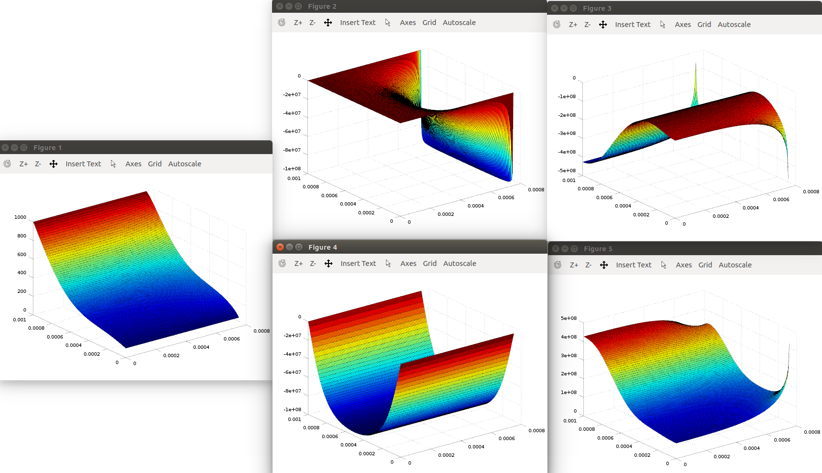
surf(xprime, yprime, T)
    
figure;
    
surf(xprime, yprime, qxout)

figure;
    
surf(xprime, yprime, qyout)

figure;
    
surf(xprime, yprime, qzout )

figure;
    
surf(xprime, yprime, sqrt(qxout.^2 + qyout.^2 + qzout.^2) )

which generates

Solution of the problem for heat equation

Limitations

Every solution method has limitations. The most noticeable limitation is that we have to perform infinity sums to get predictions using solutions from separation of variables. Infinity sums, however, cannot be performed in numerical computations, which leads us to truncate the calculations for large values of $m$, $o$, $r$, $u$, and $v$. How large these numbers have to be will depend on the problem geometry and on the material properties but, if theses number are not large enough, the calculations will manifest oscillations that will be most evident for predicted fluxes positioned near the flux boundary conditions (that is, near $x = L$ and $z = T_z$ in this solution). When observed that $m$, $o$, $r$, $u$, and/or $v$ have to be increased, a rule-of-thumb is to double their values, re-calculate the predicionts, and observe if the oscillations have decreased to acceptable intensities.

Another surprising limitation is that the flux boundary conditions at $x = L$ and $z = T_z$ are not satisfied when $y = 0$ or $y = H$. You can derivate Eqs. \ref{eq:c:solution} and \ref{eq:d:solution} with respect to $x$ and Eqs. \ref{eq:e:solution} and \ref{eq:f:solution} with respect to $z$ to observe that the term $\sin{\left(\gamma_o y\right)}$ vanishes when $y = 0$ or $y = H$ no matter what is the value of the boundary condition. The solution, however, is accurate for $y \rightarrow 0$ and $y \rightarrow H$ and the concentration/temperature is not affected by this peculiarity.

Done

Now, you can go to: