Analytical solution of the Diffusion/Heat equation in time-domain for one-dimension in cylindrical coordinates
Mar 20, 2017 by Hugo Milan
You can download the algorithm D1_HEAT_CYL_f.m for Octave/Matlab that can solve this problem here and you can see instructions in how to use it here. If you want to see the final solution, go to Solution.
In this page, we will solve the dynamic diffusion/heat equation in one-dimension using the principles of superposition and separation of variables. The problem we will solve is restricted to the following initial and boundary conditions:
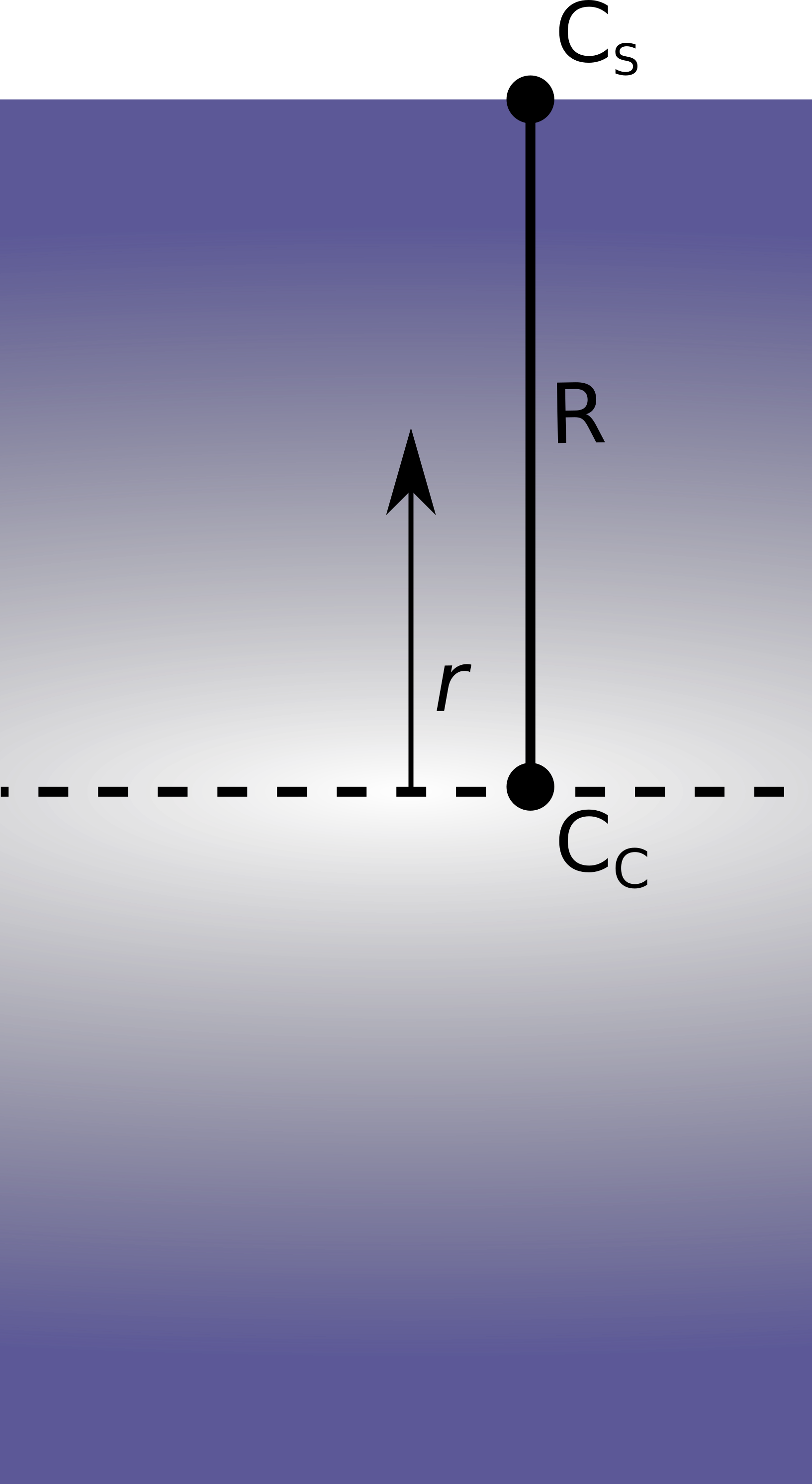
The problem geometry for the diffusion equation can be represented as shown below.
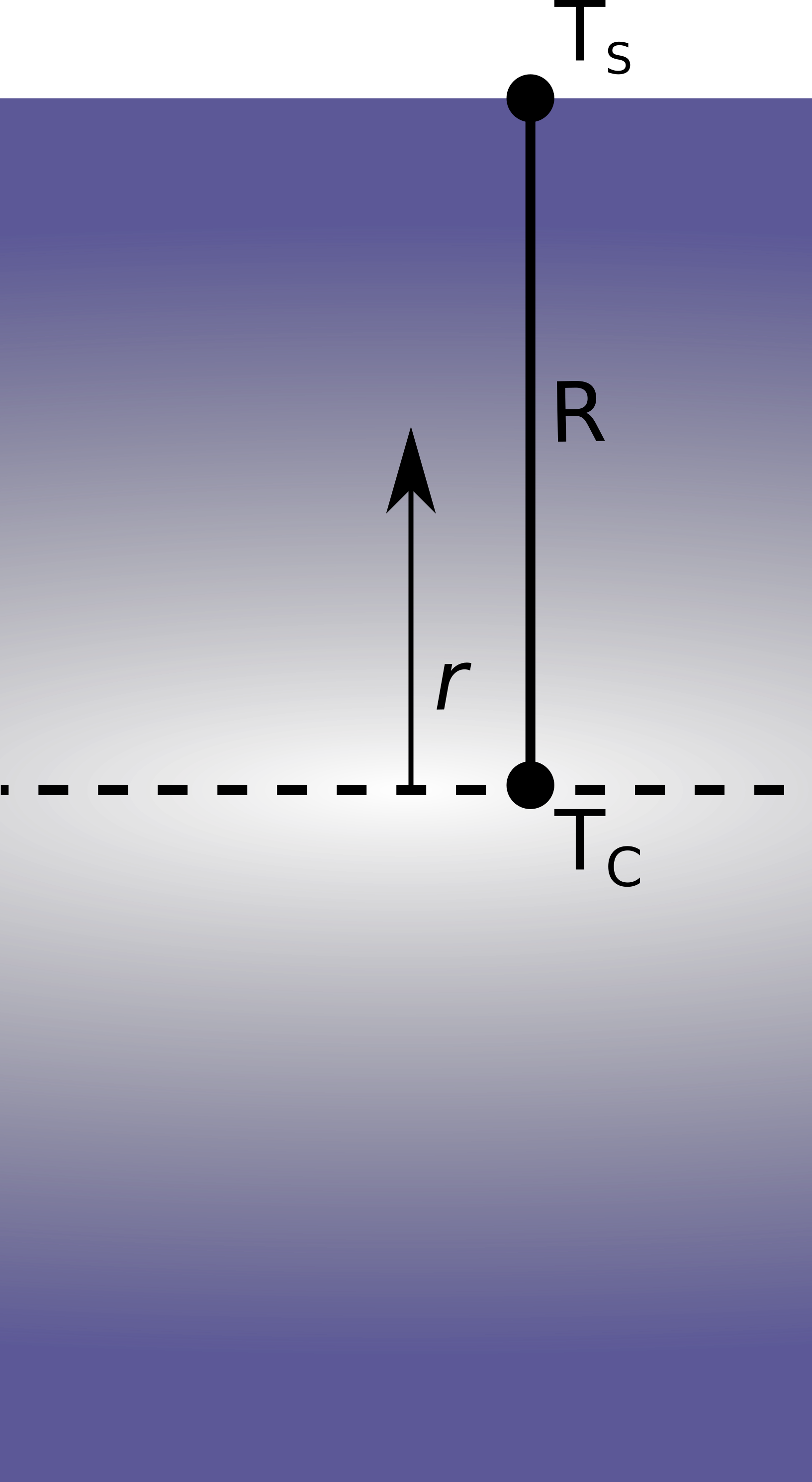
The problem geometry for the heat equation can be represented as shown below.
Governing equations
Diffusion equation:
\begin{equation} \frac{\partial C}{\partial t} = D\frac{1}{r}\frac{\partial }{\partial r}\left(r\frac{\partial C}{\partial r}\right) + S \end{equation}
where \(C\) is concentration, \(t\) is time, \(D\) is diffusivity, and \(S\) is source.
And we define the heat equation as:
\begin{equation} \rho c_{p}\frac{\partial T}{\partial t} = k\frac{1}{r}\frac{\partial }{\partial r}\left(r\frac{\partial T}{\partial r}\right) + S \label{eq:Heat} \end{equation}
where \(T\) is temperature, \(t\) is time, \(r\) is radius, \(\rho\) is density, \(c_{p}\) is specific heat, \(k\) is heat conductivity, and \(S\) is source.
Note that the diffusion equation and the heat equation have the same form when \(\rho c_{p} = 1\).
Solving
I will show the solution process for the heat equation. The solution process for the diffusion equation follows straightforwardly.
I will use the principle of suporposition so that:
\begin{equation} T(r,t) = T_c + \phi_a(r) + \phi_b(r)\tau_b(t) \label{eq:Sup} \end{equation}
and the initial and boundary conditions for these problems are:
Applying Eq. \ref{eq:Sup} in \ref{eq:Heat} yields
\begin{equation} k\frac{1}{r}\frac{\partial }{\partial r}\left(r\frac{\partial \phi_a}{\partial r}\right) + S = \rho c_{p}\phi_b\frac{\partial \tau_b}{\partial t} - k\tau_b\frac{1}{r}\frac{\partial }{\partial r}\left(r\frac{\partial \phi_b}{\partial r}\right) = 0 \end{equation}
which implies that we can solve Eqs. \ref{eq:a} and \ref{eq:b} \begin{equation} k\frac{1}{r}\frac{\partial }{\partial r}\left(r\frac{\partial \phi_a}{\partial r}\right) + S = 0 \label{eq:a} \end{equation}
\begin{equation} \rho c_{p}\phi_b\frac{\partial \tau_b}{\partial t} - k\tau_b\frac{1}{r}\frac{\partial }{\partial r}\left(r\frac{\partial \phi_b}{\partial r}\right) = 0 \label{eq:b} \end{equation}
Solving Eq. \ref{eq:a}
Equation \ref{eq:a} can be solved by direct integration, with the following general solution
\begin{equation} \phi_a = -\frac{S}{2k}y^2 + c_1 y + c_2 \end{equation}
Applying the boundary condition at \(y = 0\) we get \(c_2 = 0\). Applying the boundary condition at \(y=H\) we get: \begin{equation} c_1 = \frac{T_s - T_c}{H} + \frac{SH}{2k} \end{equation}
So, the final solution for \(\phi_a\) is:
\begin{equation} \phi_a = -\frac{S}{2k}y^2 + \left( \frac{T_s - T_c}{H} + \frac{SH}{2k} \right) y \end{equation}
Solving Eq. \ref{eq:b}
We will use separation of variables to solve Eq. \ref{eq:b}. In separation of variables, we assume that the solution is the multiplication of a function of \(y\) ( \(\phi_b(y)\) ) and \(t\) ( \(\tau_b(t)\) ). Hence,
\begin{equation} \frac{\rho c_{p}}{k\tau_b}\frac{\partial \tau_b}{\partial t} = \frac{1}{\phi_b}\frac{\partial^2 \phi_b}{\partial y^2} = -\lambda_m^2 \end{equation}
The solution of \(\phi_b\) can be expressed as:
\begin{equation} \phi_b = c_3 \sin{\left(\lambda_m y\right)} + c_4 \cos{\left(\lambda_m y\right)} \end{equation}
Applying the boundary condition at \(y = 0\) we get \(c_4 = 0\). Applying the boundary condition at \(y=H\) we get:
\begin{equation} \sin{\left(\lambda_m H\right)} = 0 \label{eq:lambdam} \end{equation}
which implies that
\begin{equation} \lambda_m = \frac{m\pi}{H} \end{equation}
with \(m = 1, 2, 3, \dotsc\) We start the counting from \(1\) because \(m = 0\) yields \(\phi_b = 0\). Now, defining \(\alpha = k/(\rho c_p) \), the solution of \(\tau_b\) is:
\begin{equation} \tau_b = c_5 \exp{\left(-\alpha\lambda_m^2 t\right)} \end{equation}
Therefore, the solution that we are looking for is:
\begin{equation} \phi_b\tau_b = \sum_{m=1}^{\infty}c_m \sin{\left(\lambda_m y\right)} \exp{\left(-\alpha\lambda_m^2 t\right)} \label{eq:b:almost} \end{equation}
Now, we apply the initial condition and get
\begin{equation} \sum_{m=1}^{\infty}c_m \sin{\left(\lambda_m y\right)} = -\phi_a = \frac{S}{2k}y^2 - \left( \frac{T_s - T_c}{H} + \frac{SH}{2k} \right) y \label{eq:b:cm} \end{equation}
To solve Eq. \ref{eq:b:cm}, we multiply both sides by an orthogonal function of the function that multiplies \(c_m\) and integrate it from \(y = 0\) to \(y = H\) to elimate the \(y\) dependence. That is, we need a function that is orthogonal to \(\sin{\left(\lambda_m y\right)}\). The function that we are looking for is \(\sin{\left(\lambda_n y\right)}\). Multiplying both sides by this function yields
\begin{equation} \int_{y=0}^{y=H}\sum_{m=1}^{\infty}c_m \sin{\left(\lambda_m y\right)}\sin{\left(\lambda_n y\right)} dy = \ldots \\ \ldots \int_{y=0}^{y=H}\left[ \frac{S}{2k}y^2 - \left( \frac{T_s - T_c}{H} + \frac{SH}{2k} \right) y \right]\sin{\left(\lambda_n y\right)} dy \label{eq:b:cm2} \end{equation}
Since we have
\begin{equation} \int_{y=0}^{y=H} \sin{\left(\lambda_m y\right)}\sin{\left(\lambda_n y\right)} dy = 0 \end{equation}
for \(m \neq n\), and
\begin{equation} \int_{y=0}^{y=H} \sin{\left(\lambda_m y\right)}\sin{\left(\lambda_n y\right)} dy = \frac{H}{2} \label{eq:mn} \end{equation}
for \(m = n\), we can drop the summation and solve Eq. \ref{eq:b:cm2} for each \(c_m\):
\begin{equation} c_m = \dfrac{\displaystyle \int_{y=0}^{y=H}\left[ \dfrac{S}{2k}y^2 - \left( \dfrac{T_s - T_c}{H} + \dfrac{SH}{2k} \right) y \right]\sin{\left(\lambda_m y\right)} dy}{ \displaystyle \int_{y=0}^{y=H}\sin^2{\left(\lambda_m y\right)} dy } \label{eq:b:cm3} \end{equation}
So, solving for the first integral,
\begin{equation} \dfrac{S}{2k}\int_{y=0}^{y=H}y^2\sin{\left(\lambda_m y\right)} dy = \dfrac{S}{2k} \frac{ \left( 2 - \lambda_m^2H^2 \right)\cos{\left(\lambda_m H\right)} + 2\lambda_m H \sin{\left(\lambda_m H\right)} - 2}{\lambda_m^3} \label{eq:b:cmf1} \end{equation}
From the definition of \(\lambda_m\) in Eq. \ref{eq:lambdam},
\begin{equation} \dfrac{S}{2k}\int_{y=0}^{y=H}y^2\sin{\left(\lambda_m y\right)} dy = \dfrac{S}{2k} \frac{ \left( -1 \right)^m \left( 2 - \lambda_m^2H^2 \right) -2 }{\lambda_m^3} \label{eq:b:cmf1b} \end{equation}
Now, solving the last integral:
\begin{equation} -\left( \dfrac{T_s - T_c}{H} + \dfrac{SH}{2k} \right)\int_{y=0}^{y=H}y\sin{\left(\lambda_m y\right)} dy = \ldots \\ \ldots -\left( \dfrac{T_s - T_c}{H} + \dfrac{SH}{2k} \right) \frac{\sin{\left(\lambda_m H\right)} - \lambda_m H\cos{\left(\lambda_m H\right)}}{\lambda_m^2} \label{eq:b:cmf2} \end{equation}
which, from the definition of \(\lambda_m\) in Eq. \ref{eq:lambdam}, becomes
\begin{equation} -\left( \dfrac{T_s - T_c}{H} + \dfrac{SH}{2k} \right) \int_{y=0}^{y=H}y\sin{\left(\lambda_m y\right)} dy = \left( -1 \right)^m\left( \dfrac{T_s - T_c}{H} + \dfrac{SH}{2k} \right) \frac{H}{\lambda_m} \label{eq:b:cmf2b} \end{equation}
From Eqs. \ref{eq:mn}, \ref{eq:b:cmf1b}, and, \ref{eq:b:cmf2b}, the final solution for \(\phi_b(y)\tau_b(t)\) is:
\begin{equation} \phi_b\tau_b = \sum_{m=1}^{\infty}\left[ \dfrac{S}{Hk} \frac{ \left( -1 \right)^m\left( 2 - \lambda_m^2H^2 \right) -2 }{\lambda_m^3} \ldots \\ \ldots + \left( -1 \right)^m\frac{2}{\lambda_m}\left( \dfrac{T_s - T_c}{H} + \dfrac{SH}{2k} \right) \right]\sin{\left(\lambda_m y\right)} \exp{\left(-\alpha\lambda_m^2 t\right)} \label{eq:b:final} \end{equation}
Solution
The final solution is:
\begin{equation} T(y,t) = T_c + \phi_a(y) + \phi_b(y)\tau_b(t) \end{equation}
with \(\alpha = k/( \rho c_p ) \), and \(\phi_a(y)\) and \(\phi_b(y)\tau_b(t)\) expressed as:
\begin{equation} \phi_a = -\frac{S}{2k}y^2 + \left( \frac{T_s - T_c}{H} + \frac{SH}{2k} \right) y \end{equation}
\begin{equation} \lambda_m = \frac{m\pi}{H} \end{equation}
\begin{equation} \phi_b\tau_b = \sum_{m=1}^{\infty}\left[ \dfrac{S}{Hk} \frac{ \left( -1 \right)^m\left( 2 - \lambda_m^2H^2 \right) -2 }{\lambda_m^3} \ldots \\ \ldots + \left( -1 \right)^m\frac{2}{\lambda_m}\left( \dfrac{T_s - T_c}{H} + \dfrac{SH}{2k} \right) \right]\sin{\left(\lambda_m y\right)} \exp{\left(-\alpha\lambda_m^2 t\right)} \end{equation}
The flux/heat flux can be obtained by derivating these equations with respect to \(y\).
Using the Algorithm
The algorithm D1_HEAT_f.m was written as a function in Octave/Matlab and you can obtain it here. To use it, you will need to define the material properties and the maximum value of \(m\).
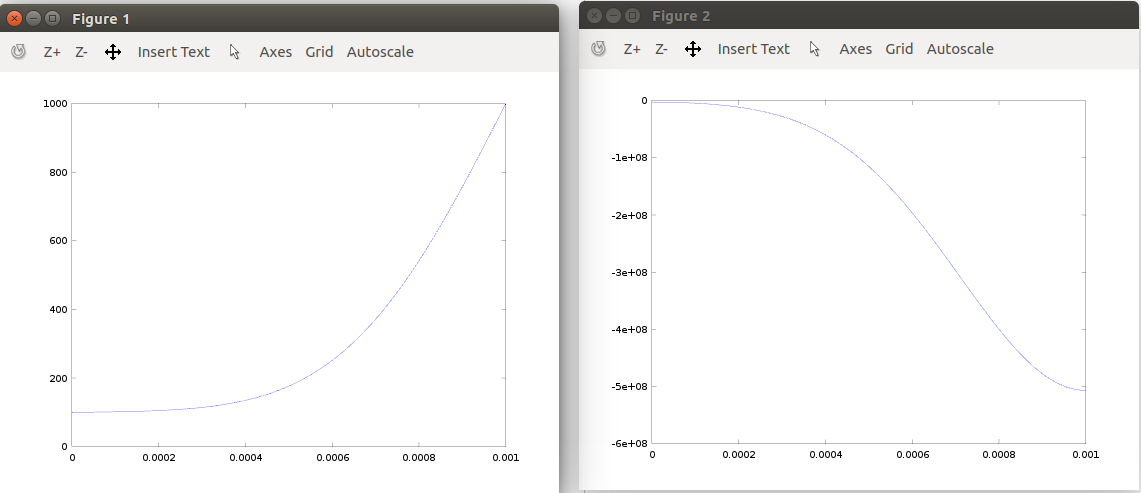
As an example, we can use the following script:
% Thermal properties
Tc = 100; % core and initial temperature (oC)
Ts = 1000; % superficial temperature (oC)
rho = 2700; % density (kg/m3)
cp = 900; % specific heat (J/(K-kg))
k = 205; % thermal conductivity (W/(K-m))
S = 5000; % internal heat source (W/m3)

% Material properties
H = 1e-3; % m
y = 0:(H/100):H;

% number of iterations of m
minf = 50;

% time of the solution
t = 0.5e-3;

[T, q] = D1_HEAT_f(y, H, t, Ts, Tc, k, rho, cp, S, minf);

plot(y, T)

figure;

plot(y, q)
which generates
Limitations
Every solution method has limitations. The most noticeable limitation is that we have to perform infinity sums to get predictions using solutions from separation of variables. Infinity sums, however, cannot be performed in numerical computations, which leads us to truncate the calculations for large values of \(m\). How large this number have to be will depend on the problem geometry and on the material properties but, if theses number are not large enough, the calculations will manifest oscillations that will be most evident for predicted fluxes. When observed that \(m\) has to be increased, a rule-of-thumb is to double its valuee, re-calculate the predicionts, and observe if the oscillations have decreased to acceptable intensities.
Done
Now, you can go to: